




An accessible guide to understanding asphalt behaviors
Fictional character Joe Miller, a lawyer played by Denzel Washington in the movie “Philadelphia” (1993), has a favorite line that he uses several times when talking to potential clients and witnesses.
“Explain it to me like I’m a 4-year-old.”
What he is saying in that short statement is “I want to understand, but I need you to simplify it quite a bit.” That resonates with us because it is a similar request that we get when discussing asphalt rheology. People want to understand but the technical terms and concepts can be daunting to them. Thus, the challenge of this article: to simplify asphalt rheology and how it relates to pavement distress in a way that can be more easily understood by industry professionals.
Unlike the imperative in the quote, we will not try to explain it as if you are four. Real four-year-olds do not want to know about asphalt rheology; they are more interested in Bluey than Black Space. But if you are willing to read on, we will do our best to show you how one picture based on two numbers can lead to a better understanding of how asphalt behaves.
Two important properties from one test
Asphalt binders are useful construction materials for pavements because in the temperature range in which they are used, they are neither 100% solid nor 100% liquid. If you push on a solid material, it resists deforming and wants to retain its original shape. That is elastic behavior. If you push on a liquid, it flows and does not try to return to its original shape when the load is removed. That is viscous behavior. At most temperatures, asphalt binder exhibits a little of both types of behavior. So how do we show that?
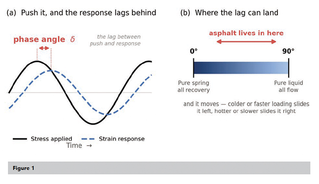
In oscillatory shear testing using a Dynamic Shear Rheometer (DSR), we twist the sample between two plates back and forth at a certain rate. That creates an input sinusoidal wave and a sample response in a corresponding output wave (Figure 1). We get stiffness by measuring how much stress the sample develops in response to the applied strain. The ratio of stress to strain is modulus, or stiffness. Because it is an oscillatory response, it includes both in-phase and out-of-phase components, meaning that it is a complex shear modulus, G*. Most often we think of this as stiffness.
But the standard DSR test also gives you an indication of how viscoelastic the binder is through an understanding of the shift between the input and response waves. If the response is purely elastic – like a spring – then the phase angle, referred to by the Greek symbol delta (δ), is zero (0) degrees. If the material response is purely viscous – like a liquid – then the phase angle (δ) is ninety (90) degrees. A phase angle between 0 and 90 degrees represents a blend of viscous and elastic behavior.
It may be commonly understood that how asphalt behaves depends on temperature. As temperature decreases, G* increases and δ decreases. Similarly, as temperature increases, G* decreases and δ increases. What is less understood is that time of loading, or rate dependence, also matters. As the rate of loading (or frequency) gets faster, G* increases and δ decreases. Similarly, as the rate of loading slows, G* decreases and δ increases. This is why a loaded dumpster parked on an asphalt pavement in the summer causes indentations while the same pavement, driven over by cars all day, stays perfectly smooth.
Rate dependence is exhibited in the creative play world through products like Thinking Putty (or for those of us of a certain age, Silly Putty). If you form a ball and throw it against a surface, it will bounce (fast loading, more elastic response) but you can set a coffee cup on it and it will flatten out (slow loading, more viscous response).
A popular picture
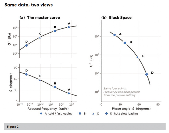
If we want to fully characterize asphalt behavior, we often test at several temperatures with different loading frequencies at each temperature. These data are then shifted using mathematical modeling to produce the resulting picture – a commonly used representation by asphalt technologists, which shows how G* can be collapsed into a single curve at a single temperature and a range of frequencies that would be impractical for lab testing (Figure 2).
A master curve is a useful tool, but it relies on frequency on the horizontal axis which often does not resonate with the understanding of the user. What does a reduced frequency of 106 rad/s even mean? Most of us do not have a practical reference for that.
Also, why do we need to look at one curve of G* versus reduced frequency and another curve of δ versus reduced frequency to understand asphalt behavior?
But maybe not the best picture
Interestingly, the Best Picture nominees for films released in 1994 included three that are now rated in the Top 20 of the all-time best according to IMDb user rankings. The most popular movie won; the higher ranked, and arguably better, films did not. “Most popular” does not necessarily mean “best.”
A master curve is an excellent picture, commonly used by asphalt technologists, of how asphalt behaves but it may not be the best picture. A better picture allows us to see how our two important properties – stiffness and viscoelasticity – relate to each other on a single graph. This kind of picture is referred to in the asphalt world as Black Space (or sometimes “Black’s Space” or “Black’s diagram”).
In Black Space, G* is plotted on a log scale on the vertical axis while δ is plotted on a linear scale on the horizontal axis. The difference between the master curve and Black Space graphs is shown in Figure 2. Specifically, in Black Space representation, the somewhat clunky “reduced frequency” goes away, leaving us with an easier understanding of how the asphalt binder behaves.
Black Space is a simple way to look at the stiffness and viscoelastic response of an asphalt binder across a wide range of temperatures and loading conditions. We can get this data from our regular DSR tests, but we will have a “curve” defined by just a few data points. A better approach, which can be automated through the operating software, is to use the same temperature-frequency sweep testing we use to generate master curves. Because each measurement already carries its own temperature and frequency, those two variables drop out of the picture entirely and the data collapse onto a single curve. One binder, one curve defining a wide range of its properties.
What Black Space does really well is show us the differences between asphalt binder properties, particularly as they become aged. For instance, two asphalt binders can have the exact same stiffness but sit in different places in Black Space, meaning the viscoelasticity is different and the expected cracking performance may also be different.
Not so much a picture as a map
How do we read a Black Space diagram? It may be useful to think of it as a map telling you where your asphalt binder has been and where it is going.
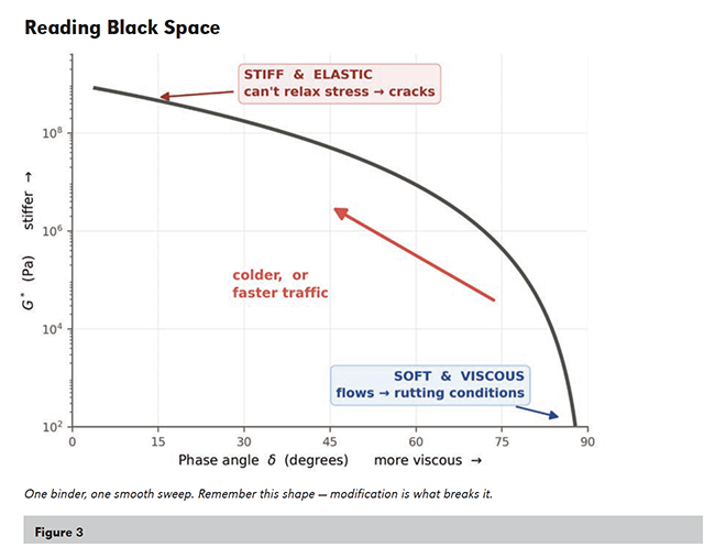
The bottom right part of the map (the “southeast”) is low stiffness and high flow (viscous) behavior. The properties in this region are what we would expect for asphalt at high temperature and slow loading. This is the region where we worry about the binder having sufficient stiffness and elastic response to minimize its contribution to rutting.
The upper left part of the map (the “northwest”) is high stiffness and more elastic/solid behavior. The properties in this region are what we would expect for asphalt at low temperature and fast loading. This is the region where we worry about the binder having stiffness that is too high and a phase angle that is too low, which leaves the binder unable to relax stresses and leads to cracking.
For a typical, unmodified asphalt binder, any DSR test at any temperature and frequency should land you on the same curve … it is just a matter of where. Colder temperatures and faster loading will move you to the northwest corner. Hotter temperatures and slower loading will move you to the southeast corner. This is illustrated in Figure 3.
Aging: moving northwest
Now that we can find our way around the map, we can start reading it. This is where the simplicity of the plot pays off. Because G* and δ appear together across the whole viscoelastic range, you can take in a binder’s behavior at a glance. This is especially helpful when assessing binder aging because as binders oxidize, they don’t just stiffen (increase G*) – they lose the ability to relax stresses (decrease δ), resulting in increased susceptibility to cracking.
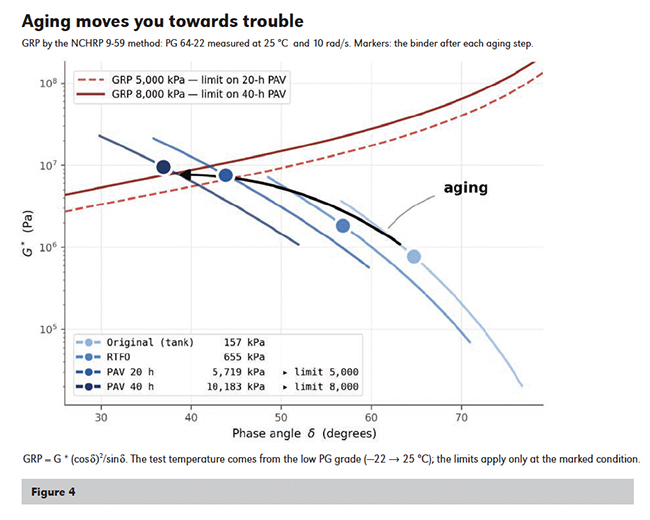
Here is where Black Space stops being theory and starts being practical. Aging effects can be assessed in two ways. First, a single point along the curve can be evaluated at a given test temperature and frequency. For example, a practitioner may consider the Glover-Rowe Parameter (GRP) measured at 10 rad/s and an intermediate grade temperature. GRP occupies a single point on the curve at a given aging condition; as aging progresses, the point on the curve moves up and to the left (northwest) along with the curve itself. Point parameters like GRP or G*sinδ are helpful for showing fatigue susceptibility with aging since they capture stiffness and phase angle response at a temperature relevant to the performance grade.
But a single point is not the whole story: we also need to look at the shape of the curve itself. In short, binder curves in Black Space tend to flatten as they move northwest with aging. That change in shape matters: as the curve gets flatter with age, increases in stiffness lead to greater decreases in phase angle. Binders in the field see temperature swings that repeatedly raise and lower their stiffness. The shape of the curve describes this temperature dependency and tells us whether the binder can still relax stress through repeated temperature cycles. Shape parameters like ΔTc, R-value and phase angle at constant modulus describe this shape, giving us a way to measure and compare binder durability in aged pavements.
Figure 4 shows a single binder moving and flattening through successive aging steps, as well as GRP points along each curve.
Modification: Bending the path
While aging shifts and flattens the curve, polymer modification bends the curve: specifically at lower stiffness (around 1 to 100 kPa), where permanent deformation is of primary concern. It’s in this region that the polymer network delivers an increased elastic response (lower phase angle), providing resistance to rutting and shoving. Polymer modification shows up in the south-southeast region of our map. The extent to which the curve bends can depend on many factors, including polymer type, polymer loading, crosslinking and base binder properties. Polymer modification comes in many forms, and so do the accompanying Black Space curves, which range from simpler ones, as shown in Figure 5, to more complicated S-curves or even curves with multiple switchbacks. Seeing polymer-modified curves in Black Space tells the story of modification beyond a single point measurement.
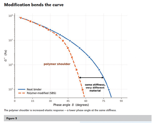
Other additives can leave signatures, too. Recycling agents (softeners and rejuvenators) can alter the curve to varying degrees. The presence of recycled asphalt materials (RAM) in a binder blend also shows up in Black Space. In this sense, the Black Space plot is a “detector” that clues practitioners into binder composition. As materials become more complex, Black Space remains a critical tool for fingerprinting asphalt materials in a clear and effective manner.
Black space in practice
The beauty of using the Black Space plot for asphalt binder characterization is that most labs already set up for AASHTO M 320 grading can do the testing with minimal additional training. Most rheometers come pre-programmed with templates for performing the frequency sweeps at multiple temperatures required to collect the data – it’s simply a matter of knowing how to select the appropriate testing parameters and how to monitor data quality. The applications are numerous: RAM characterization, forensic analysis, recycling agent evaluation, polymer response and more; Table 1 offers a brief snapshot of several applications. Researchers, agencies and testing labs should add Black Space analysis to the toolkit they use to evaluate asphalt binder and mixture behavior.
| If you want to… | Plot this | And look for |
|---|---|---|
| Distinguish between two binders of the same grade | Both candidates on one set of axes, at the same aging state. | Separation and curvature. Two PG 64-22s can meet the same grade and still sit several degrees apart in phase angle at the same stiffness. The one further west has less relaxation capacity — same grade, different product. |
| See what RAM and recycled binder do to your mix test results | Virgin binder, the recovered RAM (recycled asphalt materials) binder, and blends at each recycled content you’re considering. | Where each blend lands relative to the virgin binder and to the GRP limit. This is the binder-scale datapoint for indicating why a mixture cracking test moved when you changed the recycled content. |
| Assess binder rejuvenation versus binder softening | The aged binder before dosing, after dosing and again after re-aging the treated binder. | Direction, not just distance. A rejuvenating recycling agent alters the shape of the curve back toward its original state. The re-aged plot tells you whether the fix held. |
| Track aging on a field test project | Recovered binder from cores at construction and at years 1, 3 and 5, all on one plot. | The rate and direction of the march northwest, and where it sits against the GRP limit. Overlay lab-aged material to see whether 20-hour or 40-hour PAV actually represents your climate and your mix — that calibration is worth having before you argue about a spec limit. |
Perform forensic analysis on a failed pavement | Recovered binder from cracked and uncracked areas of the same project, plus retained original binder if anyone kept it. | Significant differences between point and shape rheology. The comparison may tell three very different stories: the binder properties were not as expected after construction, the binder aged badly in service or the problem was never the binder. |
Compare polymer blends | Base binder and each candidate modified binder, at the same aging state — then again after RTFO and PAV. | How big the polymer shoulder is and at what stiffness it engages: that is the network telling you how much polymer is doing useful work. Then check whether the shoulder survives aging. A shoulder that flattens out after PAV means the polymer degraded, which no PG grade will report. |
Fade to black
We promised to keep it simple – as best we could anyway while discussing asphalt – so we will close with a simple thought: if we want to better understand asphalt behavior as it changes with temperature, loading, aging and modification, we need to always think of two numbers (G* and δ) and one color
(“Black” space) and how they work together.
In the end, we still think a four-year-old will care more about Bluey than Black Space. But as we navigate our way through the Outback of asphalt properties, it is
good to know that with Black Space we have a map.
Cooper is the Asphalt Institute Laboratory Manager and Senior Research Scientist. Anderson is the Asphalt Institute Vice President of Research and Laboratory Services.
The origin story of Black Space, its name as a term of art and use in asphalt rheology, has been difficult to track. According to prominent researchers from the SHRP era (1988-1993), the concept apparently comes from the electrical controls world in which the magnitude of amplifiers in a control system is plotted against phase angle on a semi-log graph. In that field, it may be referred to as a Black-Nichols Chart or Black’s diagram. As our focus is on all things asphalt, the association of “Black” with “asphalt” is just too strong and we have sadly forgotten Nichols.